Much of Excel’s power and utility arises from the ability to perform complex calculations by providing one or more inputs. One example is the PMT function in Microsoft Excel, which enables us to calculate a loan payment if we provide three inputs: interest rate, loan term, and loan amount. Excel even provides a tool that walks you through crafting the formula if you haven’t created such a calculation before.
As shown in Figure 1, you’ll first need to provide three inputs: Interest Rate, Term, and then Principal (also known as the loan amount). It’s easier to write formulas in Excel if you have the inputs the formula will need in place first. From there we’ll follow the numbered steps:
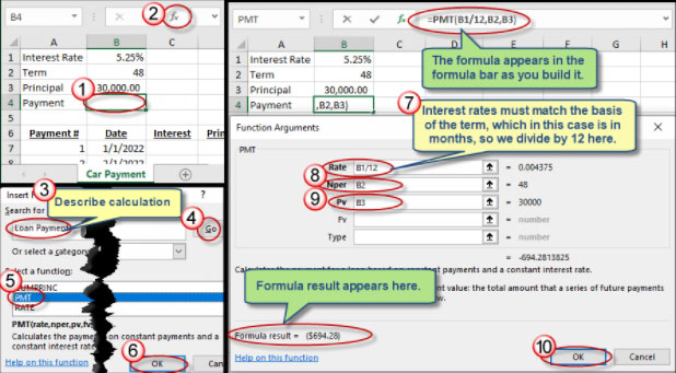
- Select the cell where you want the payment calculation to appear. Notice that you don’t need to type anything yet, just simply click on the cell.
- Click the Insert Function button on Excel’s Formula Bar, which appears above the worksheet itself. A bigger version of the Insert Function button also appears as the first command on the Formulas menu in Excel.
- Describe the calculation you’re trying to perform. If you’re contemplating buying a car, you could put Car Payment here, although as you’ll quickly see, it’s generally best to use less specific terminology, such as Loan Payment.
- Click Go. Ideally Excel will present a list of likely worksheet functions in the Select a Function listing, but if it didn’t understand the search term you entered, it may ask you to rephrase your question.
- Assuming Excel does show you a list of functions, click any function on the list and look below for what that function does. In this case Excel presents three options. CUMPRINC calculates the total principal paid on a loan between two periods, while RATE calculates the interest rate for a loan. Neither of these accomplish what we want, but the PMT function does, so select the PMT function.
- Click Go to move to the next step, which causes a Function Arguments dialog box to appear.
- The Rate field has a bolded description, which means it’s a required field. Reference your interest rate, in this case cell B1, and then divide by 12 because interest rates need to match the loan term basis. In cell B2 we provided a monthly term, so we need a monthly interest rate.
- The Nper field is where you provide the number of periods in the loan, also known as the loan term.
- The Pv field is short for Present Value, which is finance-speak for the loan amount. Money loses value over time due to inflation, and so that’s why the loan amount is referred to as the present value. Notice that the Fv (future value) and Type fields are not bolded, which means they’re optional. You can leave them blank in this case.
- Click OK to enter the formula into the worksheet cell.
If your loan amount feels incorrect, a common error is that users forget to divide the interest rate by 12. To fix this, simply click on the cell with the formula, and then click the Insert Function (fx) button again. You can use this to deconstruct worksheet function-based calculations in Excel. Once you gain more experience in Excel you’ll find it more efficient to type the formula directly into the worksheet cell, but the Function Arguments dialog box serves a bridge to help you master Excel formulas.