When you transform a list of data into a meaningful report with a few mouse clicks in Excel, pivottables can feel like a blessing. On the other hand, when duplicate values appear in that pivottable, the feature may instead feel cursed. In this article I’ll show you how to quickly resolve the issue if it arises for you in Excel. As you may expect, it’s going to be related to a nuance in your data.
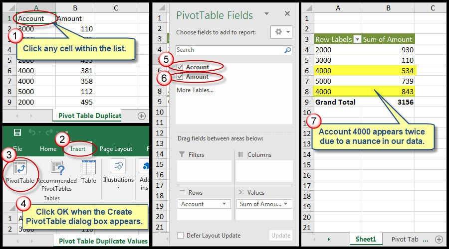
Figure 1: How to create a pivottable in Excel, and then notice the duplicate values.
As shown in Figure 1, it’s easy to create a pivot table:
- Click any cell within a list of data.
- Activate the Insert menu.
- Click the PivotTable command.
- Click OK when the Create PivotTable dialog box appears, there’s no need to make any changes in the dialog box.
- Choose a field for the Rows section, in this case we’ll use Account.
- Choose a field for the Values section, here we’ll use Amount.
- Sigh when you notice that your data is showing up on more than one row. The point of a pivottable is to consolidate data into one row for each item.
In this case the issue shown in step 7 is because some numbers are being stored as text. Fortunately Figure 2 shows an easy fix.
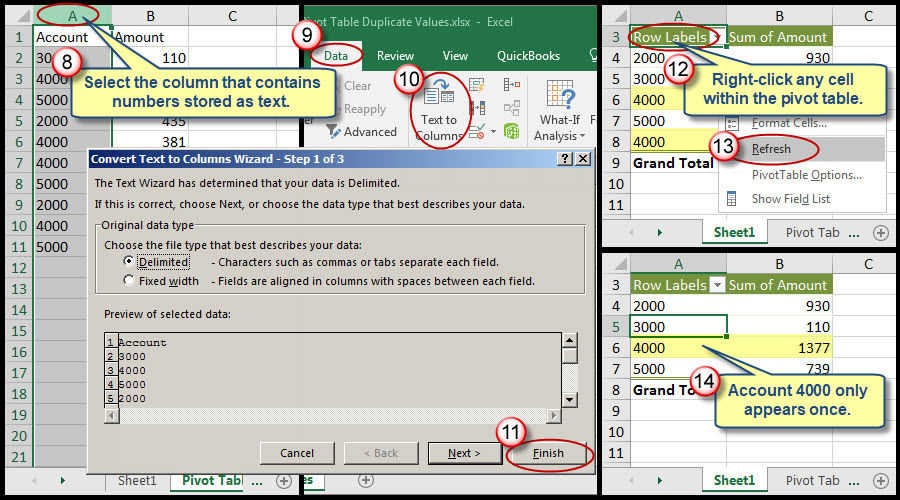
Figure 2: The Text to Columns Wizard handily resolves our text versus numbers discrepancy.Choose the column that contains numbers stored as text.
- Activate Excel’s Data menu.
- Click Text to Columns.
- In the Text to Column Wizard simply click Finish, in this context you don’t need to make any choices or work through the steps.
- Right-click any cell within the pivottable.
- Choose the Refresh command.
- Notice that now the duplicate amounts for account 4000 are consolidated into a single value.